Is climate deterministic or stochastic?
The temporal evolution of a climate simulated by a climate model is described using equations in which the time derivative of a climate variable x equals the responsible dynamical forcing f and hence satisfying satisfying dx / dy = f . The time derivative operator is a high-pass filter. This has a severe consequence for the internal climate variability on ultra-long timescales. Contrary to common understanding, Prof. von Storch shows that this long-timescale variability cannot be deciphered from the responsible internal dynamics on the same timescales.
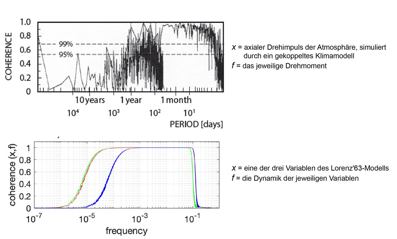
The author draws her conclusion for a climate in an equilibrium state reached under a constant external forcing, based on a meticulous decomposition of the total equilibrium variance in terms of spectra, and supported by the spectra derived from the Lorenz model (Lorenz, 1963) as a simple climate toy-model. On the one hand, the time derivative operator suppresses variations of the internal dynamics on ultra-long timescales, consistent with the fact that internal dynamics operate only on finite timescales (since otherwise no equilibrium state can be reached). On the other hand, an equilibrium climate solution varies on all timescales, including the infinite timescales, since (when left alone with the same constant external forcing) the equilibrium solution varies stationarily into infinite times. Thus, the spectrum of a climate variable x on almost-infinite and infinite timescales is white and not zero, whereas the spectrum of the responsible dynamical forcing f is de facto zero on almost-infinite timescales and vanishes exactly on infinite timescales, leading to a breakdown of coherence between x and f on ultra-long timescales (see figure).

Fig.: Coherence spectra between x and f for two dynamical systems - a coupled model (top) and the Lorenz’ 63 model (bottom) - and for the first, second, and third component for the Lorenz model (green, red, and blue, bottom). Each of the considered dynamical systems is described by a multidimensional state vector x. For the coupled model, x is the axial angular momentum of the atmosphere and hence a function of x. For the Lorenz model, x is a component of x. In both cases, f = f (x) is the dynamics determining the evolution of x via dx / dt = f.
The missing link between a climate variable x and its dynamical forcing f on ultra-long timescales makes room for another variance-generation mechanism — the integral effect — to be effective. This mechanism cannot be expressed in terms of f at individual time instances. It only unfolds when integrating the equations forward in time, and has to be stochastically represented, for instance in terms of Hasselmann’s stochastic climate model (Hasselmann, 1976). From the point of view that a physical phenomenon, such as internal climate variability on ultra-long timescales, cannot be governed by two different types of evolution laws, one formulated in terms of deterministic differential equations and the other in terms of stochastic differential equations, the powerlessness of f suggests that a stochastic model (once identified) should not be considered as an approximation, but should be “upgraded” to something having the same status as the deterministic evolution laws represented in terms of f.
Original publication
von Storch, J. S. (2022). On equilibrium fluctuations. Tellus A, 74, 364-381. doi: 10.16993/tellusa.25
Further Information
Hasselmann, K. (1976). Stochastic climate models: Part 1. Theory. Tellus, 28, 473-485. doi: 10.3402/tellusa.v28i6.11316
Contact
Prof. Jin-Song von Storch
Max Planck Institute for Meteorology
Email: jin-song.von.storch@mpimet.mpg.de
