Fully coupled climate-ice sheet simulations of the last deglaciation
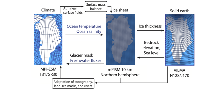
The climate system has undergone dramatic changes during the last deglaciation from 21,000 years before present to present day. For example, the Laurentide ice sheet over North America and the Fennoscandian ice sheet over Northern Europe have completely disappeared. This collapse of the ice sheets was accompanied by a global sea-level rise of ~120 m. The individual climate components and their responses to changing conditions are closely intertwined with each other. To account for feedback processes between the single climate components, such as e.g. ice-sheet retreat, freshwater input into the ocean, and the associated sea-level rise, necessitates the application of a fully coupled modeling framework with interactive ice sheets in which each of the climate components is comprehensively modeled. To represent these interactions in our simulations, we have developed a fully coupled climate-ice sheet model, consisting of the latest version of MPI-ESM for the atmosphere, land, and ocean, the ice sheet model mPISM, and the solid-earth model VILMA (Fig. 1). We have also added an Eulerian iceberg module. In addition, modules for an automated computation of bathymetry and land-sea mask changes in response to sea-level changes (Meccia et al., 2018), and, in collaboration with the department of Land in the Earth System, automated river routing (Riddick et al., 2018) have also been added. All of the latter modules allow to simulate processes within the climate system that can have a significant impact on the climate, as they alter the global heat transport.
The primary research goal is to achieve a plausible deglaciation scenario with the fully coupled model that is in accordance with proxy data observations and to extent these simulations into the future to investigate potential future climate instabilities. For the deglaciation, this means that over the course of the simulation all of the northern hemisphere ice sheets retreat and disappear with the exception of the Greenland ice sheet. For the Antarctic ice sheet we expect a clear ice volume reduction in comparison to the last glacial maximum. Moreover, important climate events such as meltwater pulses associated with a sudden retreat of the ice sheets should be captured by the model.
To achieve such globally plausible deglaciation simulations, we face several challenges. Computational limitations for such long-term simulations dictate that compromises have to be made, e.g. that coarse to moderate resolution has to be employed for every model component (e.g. T31 for the atmosphere, GR30 for the ocean). Considering the differing ice-sheet response in terms of timing and magnitude in the northern and southern hemisphere during this period, we further need to find a set of model parameters that works for both hemispheres during the model tuning.
To speed-up computations, we perform most of the tuning in an asynchronously coupled model setup. In this setup, we run the computationally most expensive model components, which are atmosphere and ocean, for 10 years. The cheaper model components, such as the ice-sheet and solid-earth models, are run for 100 years but use repeated forcing from the shorter atmosphere-ocean simulation. The advantage of asynchronous coupling is that it allows us to perform many simulations to test different parameter ranges. The drawback of this type of coupling is that in periods of rapid climate variations, the response of slowly reacting model components (e.g. ocean) is not fully captured. This means that final model fine tuning can only be done within the synchronously coupled model.
In the asynchronous coupled model setup, we have found a set of parameters that works for both hemispheres and provides a plausible scenario of the last deglaciation. The main ice sheets in the northern hemisphere retreat and disappear with only the Greenland ice sheet remaining until today. In the south, the Antarctic ice sheet extends at the Last glacial maximum almost all the way to the continental shelf before it starts to retreat to its present-day geometry. While the main retreat mechanism in the north is a warming climate with a corresponding increase in ice melt, the retreat of the Antarctic ice sheet is primarily driven by warming ocean waters that thin the ice from underneath. Our simulation is also able to reproduce most of the extreme climate events associated with the last deglaciation such as meltwater pulses and Heinrich events.
Contacts: Olga Erokhina, Marie Kapsch, Uwe Mikolajewicz, Clemens Schannwell
References:
Meccia, V. L. and Mikolajewicz, U.: Interactive ocean bathymetry and coastlines for simulating the last deglaciation with the Max Planck Institute Earth System Model (MPI-ESM-v1.2). Geoscientific Model Development, 11, 4677-4692, http://dx.doi.org/10.5194/gmd-11-4677-2018, 2018.
Riddick, T., Brovkin, V., Hagemann, S. and Mikolajewicz, U.: Dynamic hydrological discharge modelling for coupled climate model simulations of the last glacial cycle: the MPI-DynamicHD model version 3.0. Geoscientific Model Development, 11, 4291-4316. http://dx.doi.org/10.5194/gmd-11-4291-2018, 2018.